XRF Web Seminar Module 2 – Basic XRF Concepts
2-1
Module 2:
Basic XRF Concepts
August 2008 2-1
Module 2 – Basic XRF Concepts XRF Web Seminar
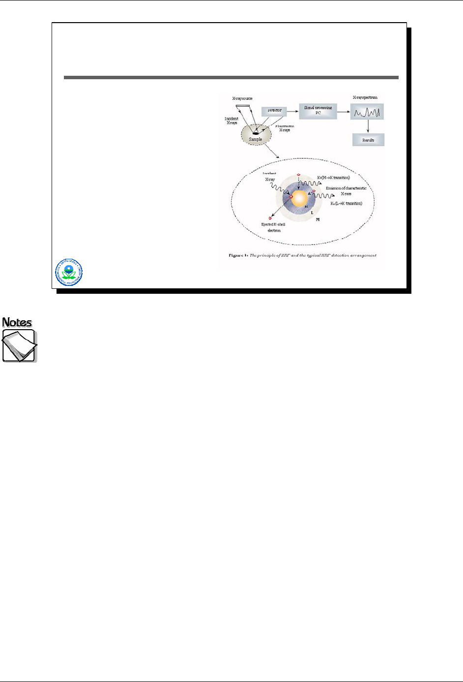
What Does An XRF Measure?
X-ray source irradiates
sample
Elements emit
characteristic x-rays in
response
Characteristic x-rays
detected
Spectrum produced
(frequency and energy
level of detect x-rays)
Concentration present
estimated based on
sample assumptions
Source: http://omega.physics.uoi.gr/xrf/english/images/PRINCIP.jpg
2-2
X-ray source irradiates sample: Modern XRF systems include basically three
components: an x-ray source, a detector, and a signal processing unit. The x-
ray source produces x-rays that irradiate the sample of interest. Traditionally x-
ray sources were sealed radionuclide sources such as Fe-55, Cd-109, Am-241,
or Cm-244. Each sealed source type emitted x-rays of a particular energy level.
The selection of a sealed source depended on the elements of interest, since
different elements respond best to different irradiating x-ray energy levels.
Sealed sources, however, presented practical challenges: some had relatively
short half-lives meaning that they had to be changed on a regular basis to
maintain XRF performance; they often required special licenses to be used; and
each only addressed a relative small set of inorganic contaminants of concern.
Consequently manufacturers of XRF units have been moving to electronic x-ray
tubes for producing the required x-rays.
Elements emit characteristic x-rays in response: When a sample is irradiated
with x-rays, the x-rays interact with individual atoms, and these atoms respond by
“fluorescing”, or producing their own x-rays whose energy levels and abundance
(number) are different for each element.
Characteristic x-rays detected: The XRF detector captures these fluorescent
x-rays, counting each and identifying their energy levels.
Spectrum produced (frequency and energy level of detect x-rays): The
signal processing unit takes the detector information and produces spectrum.
Additional software processing converts the spectrum into element-specific
estimates of the concentrations present.
August 2008 2-2

XRF Web Seminar Module 2 – Basic XRF Concepts
Concentration present estimated based on assumptions: Additional
software processing converts the spectrum into element-specific estimates of the
concentrations present based on sample assumptions.
August 2008 2-3
Module 2 – Basic XRF Concepts XRF Web Seminar
2-3
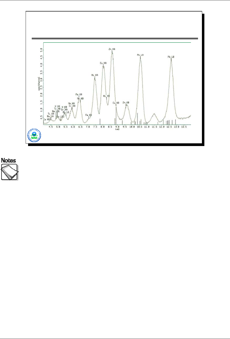
Example XRF Spectra
This slide shows an example of an x-ray spectra produced by an XRF
measurement. The x-axis is x-ray energy, and the y-axis shows the number of x-
rays observed at each energy level. The peaks are indicative of the presence of
unique elements. The heights of the peaks are proportional to the number of x-
rays counted, which in turn is proportional to the mass of the element present in
the sample. The width of the peaks, in general, is an indication of the detector’s
ability to “resolve” x-ray energies it observes, or in other words, to correctly
identify the energy level of the x-ray it detected. The better the resolution, the
tighter these peaks will be, the better the XRF will be in terms of performance
(i.e., correctly identifying and quantifying the presence of a particular element).
This spectrum has a couple of features of interest. As this spectrum
demonstrates, any particular element can have more than one peak associated
with it, for example lead, or zinc, or iron in this spectrum. As this spectrum also
demonstrates, peaks for individual elements may be so close that for all practical
purposes they are indistinguishable. The Fe/Mn peak around 6.5 KeV is a good
example. This is what causes what is known as interference, which is something
that will be discussed later.
August 2008 2-4
XRF Web Seminar Module 2 – Basic XRF Concepts
2-4
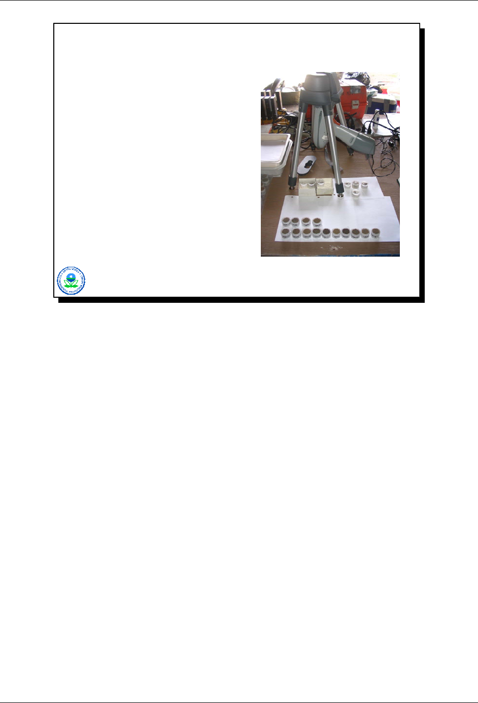
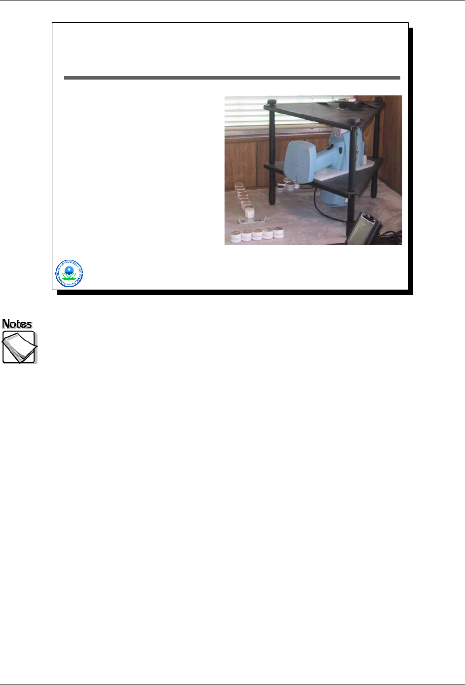
Bench-top XRF
This slide shows a bench-top XRF unit. Samples from the field are brought to
the unit which can be located in a trailer. XRF is a well-established analytical
technique with a long history of use in a laboratory environment. In the last
decade advances in electronics have allowed the development and refinement of
field-deployable units. XRF analysis is different from most other inorganic
techniques in that it is a non-destructive analysis. In other words, the original
sample is not destroyed by the analytical process. There are no extraction or
digestion steps. Consequently the same material can be analyzed repeatedly by
an XRF unit, or analyzed by an XRF unit and then submitted for some other
analysis.
August 2008 2-5
Module 2 – Basic XRF Concepts XRF Web Seminar
How is an XRF Typically Used?
Measurements on
prepared samples
Measurements
through bagged
samples (limited
preparation)
In situ measurements
of exposed surfaces
(continued)
2-5
Measurements on prepared samples: The XRF can be used to take
measurements on samples that are prepared by drying and grinding. The
sample measured consists typically of a few grams of soil contained in a special
cup designed for XRF use.
Measurements through bagged samples (limited preparation): The XRF can
also be used to take measurements on bagged samples that have undergone
very little preparation.
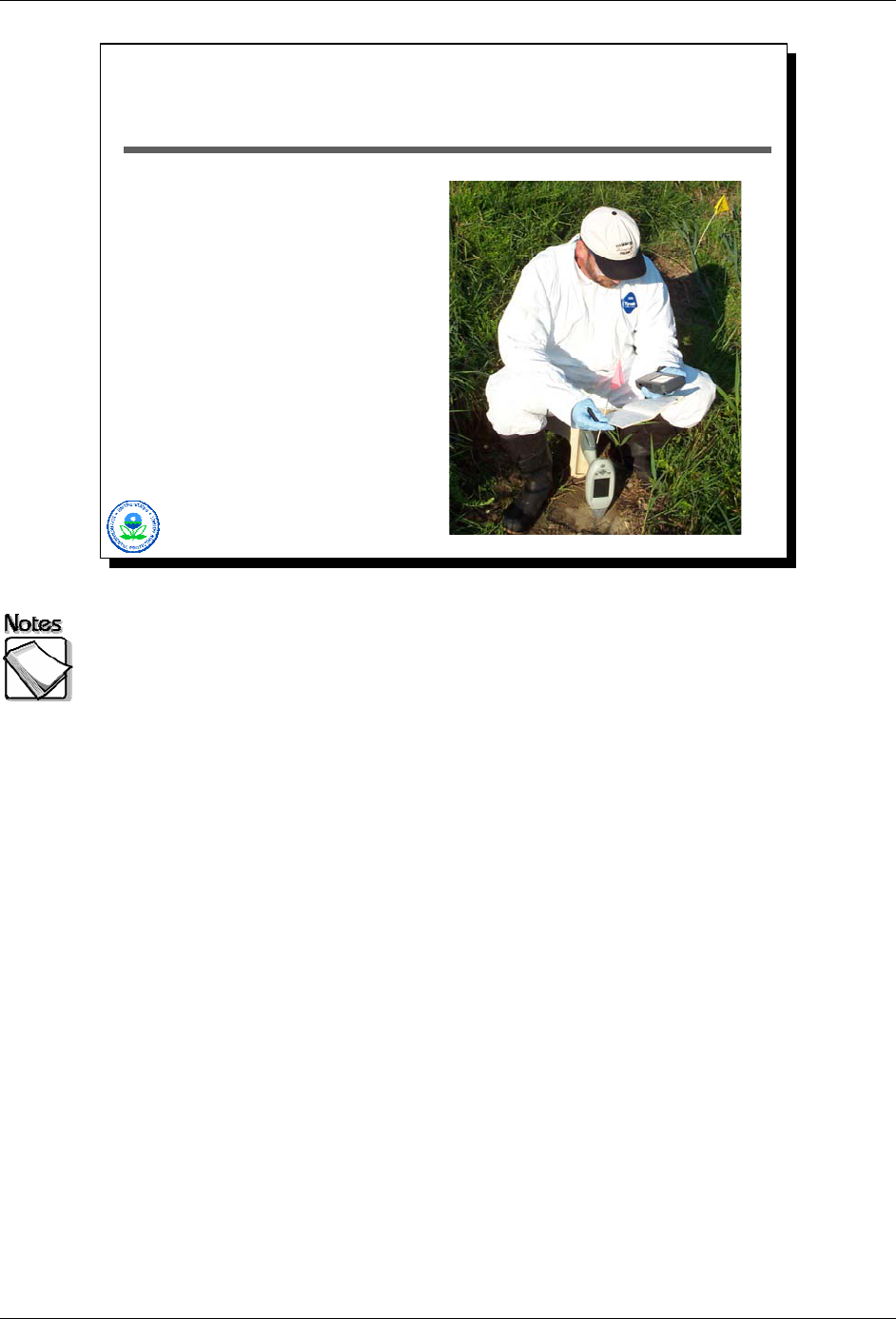
In situ measurements of exposed surfaces: The XRF can also be used to
take measurements of exposed surfaces in the field. Only surface
measurements can be made using this method.
August 2008 2-6
XRF Web Seminar Module 2 – Basic XRF Concepts
How is an XRF Typically Used?
Measurements on
prepared samples
Measurements
through bagged
samples (limited
preparation)
In situ measurements
of exposed surfaces
2-6
Measurements on prepared samples: The XRF can be used to take
measurements on samples that are prepared by drying and grinding. The
sample measured consists typically of a few grams of soil contained in a special
cup designed for XRF use.
Measurements through bagged samples (limited preparation): The XRF can
also be used to take measurements on bagged samples that have undergone
very little preparation.
In situ measurements of exposed surfaces: The XRF can also be used to
take measurements of exposed surfaces in the field. Only surface
measurements can be made using this method.
August 2008 2-7
Module 2 – Basic XRF Concepts XRF Web Seminar
What Does an XRF Typically Report?
Measurement date
Measurement mode
“Live time” for measurement acquisition
Concentration estimates
Analytical errors associated with estimates
User defined fields
2-7
What does an XRF typically report: The following items are typically reported
by the XRF:
» Measurement date
» Measurement mode – which includes the type of sample measured
» “Live time” for measurement acquisition – which indicates the number of
seconds the detector was actually collecting information. This is a subtle but
important point. In the case of Innov-X instruments, a measurement time is
selected and the measured acquired for that duration. The live time for an
Innov-X unit is something less (typically 80%) than the measurement time. In
contrast, for a Niton instrument the measurement time selected by the user
corresponds to the live time, and consequently a Niton measurement will
actually take longer than specified measurement time (typically around 20%
longer).
» Concentration estimates. Consistent with SW846 Method 6200, a “<LOD” is
typically reported when the measured result is less than 3 times the standard
deviation for that measurement as estimated by the instrument. For both
Niton and Innov-X, the software can be set to force the instrument to report
measured values no matter their error. The pros and cons of doing this will
be discussed later.
August 2008 2-8

XRF Web Seminar Module 2 – Basic XRF Concepts
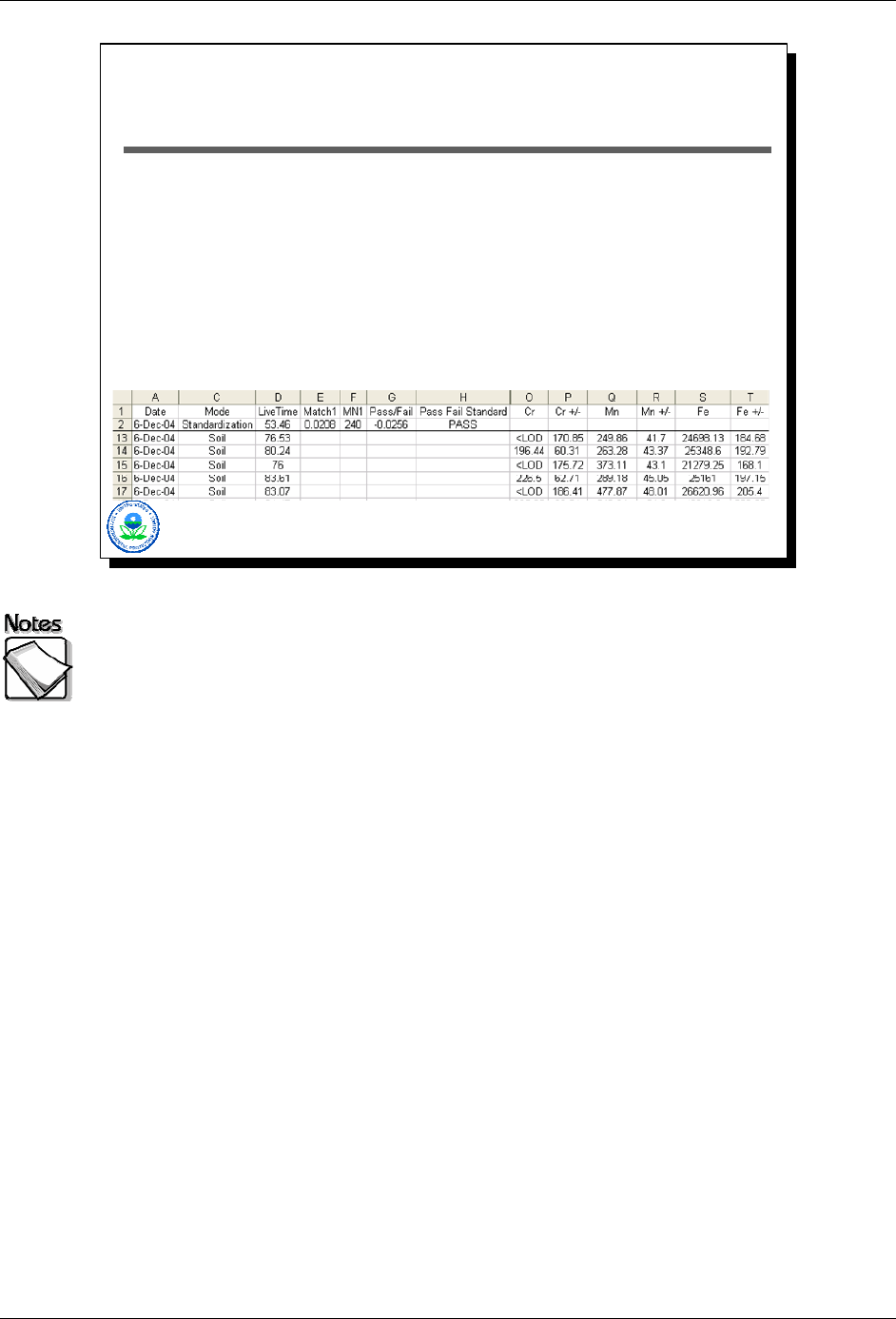
» Analytical errors associated with estimates. Two important notes here. In the
case of an Innov-X unit, the reported error is an estimate of the one standard
deviation error associated with the reported value. In the case of a Niton unit,
the reported error is actually twice the estimated standard deviation error
associated with the measurement. For both instruments, if a <LOD is
reported as a result, the error column will contain the estimated detection limit
for that measurement rather than the error. The estimated detection limit is
three times the error. One can see this in the case of Cr. The first
measurement reports Cr as an <LOD with a detection limit of 170 ppm. The
second measurement reports Cr as 196 ppm with an error that is
approximately a third of the detection limit reported by the previous
measurement.
» User defined fields – which may include comparison to a certain
concentration
August 2008 2-9

Module 2 – Basic XRF Concepts XRF Web Seminar
Which Elements Can An XRF
Measure?
Generally limited to elements with atomic number
> 16
Method 6200 lists 26 elements as potentially
measurable
XRF not effective for lithium, beryllium, sodium,
magnesium, aluminum, silicon, or phosphorus
In practice, interference effects among elements
can make some elements “invisible” to the
detector, or impossible to accurately quantify
2-8
Generally limited to elements with atomic number > 16: The XRF is
generally limited to elements which have an atomic number greater than 16.
However, the XRF cannot necessarily measure all elements with an atomic
number greater than 16 at concentrations that would be considered acceptable
for environmental applications.
Method 6200 lists 26 elements as potentially measurable: EPA Method 6200
for Field Portable X-Ray Fluorescence Spectrometry lists the following elements
as being potentially measurable:
» Antimony (Sb)
» Arsenic (As)
» Barium (Ba)
» Cadmium (Cd)
» Calcium (Ca)
» Chromium (Cr)
» Cobalt (Co)
» Copper (Cu)
» Iron (Fe)
» Lead (Pb)
» Manganese (Mn)
» Mercury (Hg)
» Molybdenum (Mo)
» Nickel (Ni)
» Potassium (K)
» Rubidium (Rb)
» Selenium (Se)
2-10 August 2008

XRF Web Seminar Module 2 – Basic XRF Concepts
» Silver (Ag)
» Strontium (Sr)
» Thallium (Tl)
» Thorium (Th)
» Tin (Sn)
» Titanium (Ti)
» Vanadium (V)
» Zinc (Zn)
» Zirconium (Zr)
XRF not effective for lithium, beryllium, sodium, magnesium, aluminum,
silicon, or phosphorus: The XRF cannot detect common elements that are
considered to be “light” elements, such as lithium, beryllium, sodium,
magnesium, aluminum, silicon, and phosphorus.
In practice, interference effects among elements can make some elements
“invisible” to the detector, or impossible to accurately quantify: In practice,
the performance of the XRF (as measured by detection limits and ability to
accurately quantify an element) is highly variable from element to element. One
of the factors contributing to variations in performance is the interference among
elements whereby the elevated presence of one element may mask the elevated
presence of another. A common example is arsenic being masked by the
presence of lead. Interference effects are real, element-specific, and at times
significant.
August 2008 2-11

Module 2 – Basic XRF Concepts XRF Web Seminar
How Is An XRF Calibrated?
Fundamental Parameters Calibration – calibration
based on known detector response properties,
“standardless” calibration, what is commonly done
Empirical Calibration – calibration calculated using
regression analysis and known standards, either site-
specific media with known concentrations or prepared,
spike standards
In both cases, the instrument will have a dynamic range
over which a linear calibration is assumed to hold.
2-9
Most, in not all, XRF vendors today are more than happy to help users develop
site-specific calibrations for their XRF applications. These can be particularly
important where site-specific matrix effects are of particular concern, and/or
when the element of interest is not one of the standard set used for factory
standardless calibrations.
It is important to remember that the XRF is no different than any other analytical
method. Properly calibrated, it will have a range of concentrations over which the
linear calibration is assumed to hold for any particular element. That range
typically runs from the instrument’s detection limits up to the percent range of
concentrations. One should not expect the XRF to accurately report
concentrations above its calibration range. In a standard laboratory the solution
to this problem is to dilute the sample. Unfortunately dilution is not an option with
a field-deployed XRF. The issue of calibration range is typically not a problem if
one is simply screening soils for concentrations above or below some decision-
making threshold. It can become an issue, however, if one is interested in
estimating the average concentration over an area using multiple XRF
measurements, and when some of those measurements include high levels of
contamination. It can also be an issue when one is trying to establish
comparability between an XRF result and a corresponding laboratory analysis,
and that comparison involves highly contaminated samples.
2-12 August 2008
XRF Web Seminar Module 2 – Basic XRF Concepts
2-10
Dynamic Range a Potential Issue
No analytical method is
good over the entire range
of concentrations
potentially encountered
with a single calibration
XRF typically under-
reports concentrations
when calibration range
has been exceeded
Primarily an issue with
risk assessments
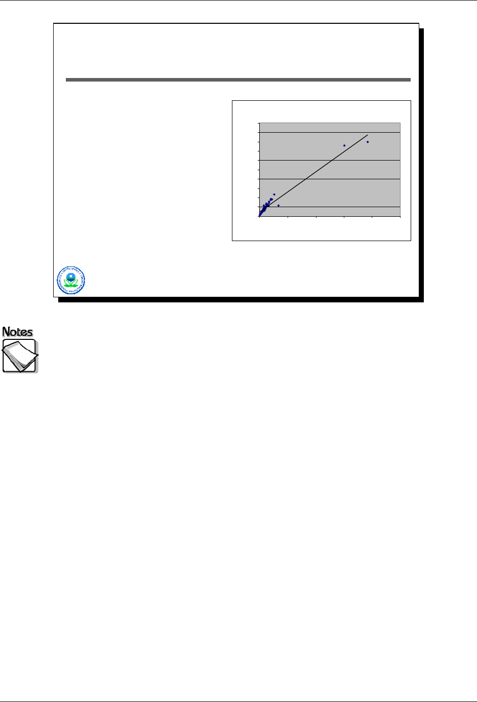
Figure 1: ICP vs XRF (lead - all data)
y = 0.54x + 200
R
2
= 0.95
0
500
1000
1500
2000
2500
3000
3500
4000
4500
5000
0 2000 4000 6000 8000 10000
ICP Lead ppm
XRF Lead ppm
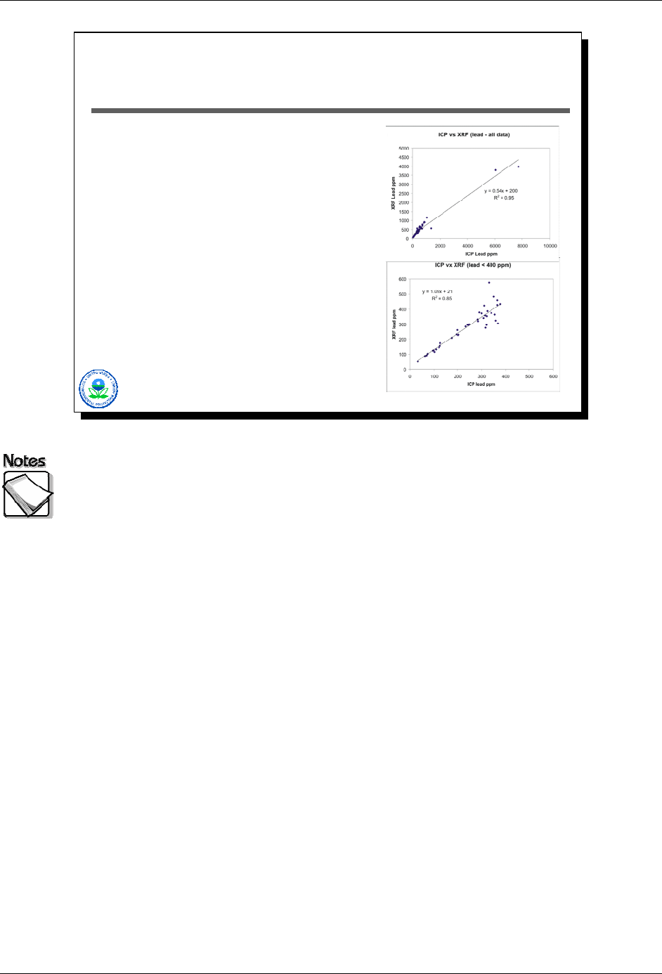
No analytical method is good over the entire range of concentrations
potentially encountered with a single calibration: As the graph shows, there
is good agreement between the XRF and ICP analysis at the lower end of the
concentration range but not at the higher end of the concentration range.
XRF typically underreports concentrations when calibration range has
been exceeded: As the graph shows, the XRF reports lower concentrations of
lead than the ICP analysis at concentrations above 6,000 parts per million (ppm).
Primarily an issue with risk assessments: This phenomenon is an issue
when the data are to be used in a risk assessment because underreporting
concentrations may underestimate the actual risk associated with the
contamination.
August 2008 2-13

Module 2 – Basic XRF Concepts XRF Web Seminar
Standard Innov-X Factory
Calibration List
Antimony (Sb) Iron (Fe) Selenium (Se)
Arsenic (As) Lead (Pb) Silver (Ag)
Barium (Ba) Manganese (Mn) Strontium (Sr)
Cadmium (Cd) Mercury (Hg) Tin (Sn)
Chromium (Cr) Molybdenum (Mo) Titanium (Ti)
Cobalt (Co) Nickel (Ni) Zinc (Zn)
Copper (Cu) Rubidium (Ru) Zirconium (Zr)
2-11
This slide shows the list of compounds available for the standard Innov-X factory
calibrations.
2-14 August 2008

XRF Web Seminar Module 2 – Basic XRF Concepts
How Is XRF Performance Commonly
Defined?
Bias – does the instrument systematically under or over-
estimate element concentrations?
Precision – how much “scatter” solely attributable to
analytics is present in repeated measurements of the
same sample?
Detection Limits – at what concentration can the
instrument reliably identify the presence of an element?
Quantitation Limits – at what concentration can the
instrument reliably measure an element?
Representativeness – how representative is the XRF
result of information required to make a decision?
Comparability – how do XRF results compare with
results obtained using a standard laboratory technique?
2-12
How is XRF performance commonly defined: The following factors are used
to define how an XRF performs:
» Bias – does the instrument systematically under or over-estimate element
concentrations?
» Precision – how much “scatter” solely attributable to analytics is present in
repeated measurements of the same sample?
» Detection Limits – at what concentrations can the instrument reliably identify
the presence of an element?
» Quantitation Limits – at what concentrations can the instrument reliably
measure an element?
» Representativeness – how representative is the XRF result of information
required to make a decision?
» Comparability – how do XRF results compare with results obtained using a
standard laboratory technique?
The following slides will discuss precision, detection limits, and comparability in
more detail.
August 2008 2-15

Module 2 – Basic XRF Concepts XRF Web Seminar
Analytical Precision Driven By…
Measurement time – increasing measurement
time reduces error
Element concentration present – increasing
concentrations increase error
Concentrations of other elements present –as
other element concentrations rise, general
detection limits and errors rise as well
2-13
Measurement time: Measurement time affects precision. Increasing the
measurement time reduces error and increases precision.
Element concentration present: The amount of the element of concern affects
precision. Generally, increasing concentrations result in increased error and
decreased precision.
Concentrations of other elements present: The presence of other elements
affects precision. As the concentration of other elements rise, general detection
limits and errors rise, decreasing analytical precision.
2-16 August 2008
XRF Web Seminar Module 2 – Basic XRF Concepts
2-14
Lead Example: Concentration Effect
Reported Error vs. Lead Concentrations
0
10
20
30
40
50
60
70
80
0 500 1000 1500 2000 2500 3000
XRF Lead Concentrations (ppm)
Reported Error (ppm)
The next two slides show two graphs that illustrate the effects of concentrations
on reported measurement errors in the case of 434 lead measurements with an
XRF. In the first graph, the x-axis shows lead concentrations while the y-axis
shows their associated reported errors. One gets the general relationship that
one would expect: error grows as the square root of concentration. In other
words, to double the error one needs to quadruple the concentration.
Notice too that these relationships start to fall apart as XRF lead values become
high, reflecting the contribution of other sources of error to measurement error
(e.g., the presence of other elements that are very elevated).
August 2008 2-17
Module 2 – Basic XRF Concepts XRF Web Seminar
2-15
Lead Example: Concentration Effect
% Error vs. Lead Concentrations
0
5
10
15
20
25
30
35
0 500 1000 1500 2000 2500 3000
XRF Lead Concentrations (ppm)
% Error
This graph also illustrates the effects of concentrations on reported measurement
errors in the case of 434 lead measurements with an XRF. Percent error is
plotted as a function of concentration. Notice that % error is a maximum at the
detection limits of the instrument, and is never more than approximately 30%.
For lead values in the range of what is typically of interest (e.g., 400 ppm),
percent error is less than 5%. This is an important fact to keep in mind. The
expectation for standard laboratory analytical precision is less than 10%. In the
case of this XRF example, the XRF meets that expectation for lead values
greater than approximately 100 ppm. A general rule of thumb for any particular
element is that for concentrations that are10 times the XRF’s detection limit, the
analytical error of XRF measurements will be less than 10%.
2-18 August 2008

XRF Web Seminar Module 2 – Basic XRF Concepts
XRF Detection Limit (DL)
Calculations
SW-846 Method 6200 defines DL as 3 X the
standard deviation (SD) attributable to the
analytical variability (imprecision) at a low
concentration
XRF “measures” by counting X-ray pulses
XRF instruments typically report DLs based on
counting statistics using the 3 X SD definition
SDs and associated DLs can also be calculated
manually from repeated measurements of a
sample (if concentrations are detectable to begin
with)
2-16
XRF detection limit (DL) calculations: Remember that relative error or percent
error (error divided by the concentration) falls as concentration increases. What
this means is that using this definition of detection limits, the percent error
associated with an XRF measurement will never be more than approximately
30%, and usually will be significantly less.
A common question people ask is what the detection limit is for a measurement
where the element of interest was detected and reported by the XRF. A common
mistake is for the detection limit to be estimated, in this case, by taking the error
of the measurement and multiplying the error by three. This can significantly
over-estimate the detection limits of the instrument. The reason is that analytical
error increases as concentrations increase. Consequently the error for a
quantifiable concentration will be greater than the error if the element had not
been present.
August 2008 2-19

Module 2 – Basic XRF Concepts XRF Web Seminar
2-17
The 3 Standard Deviation Concept
Frequency of XRF Responses When Element Not Present
Stdev = 5 ppm
Detection Limit:
15 ppm
99.87%
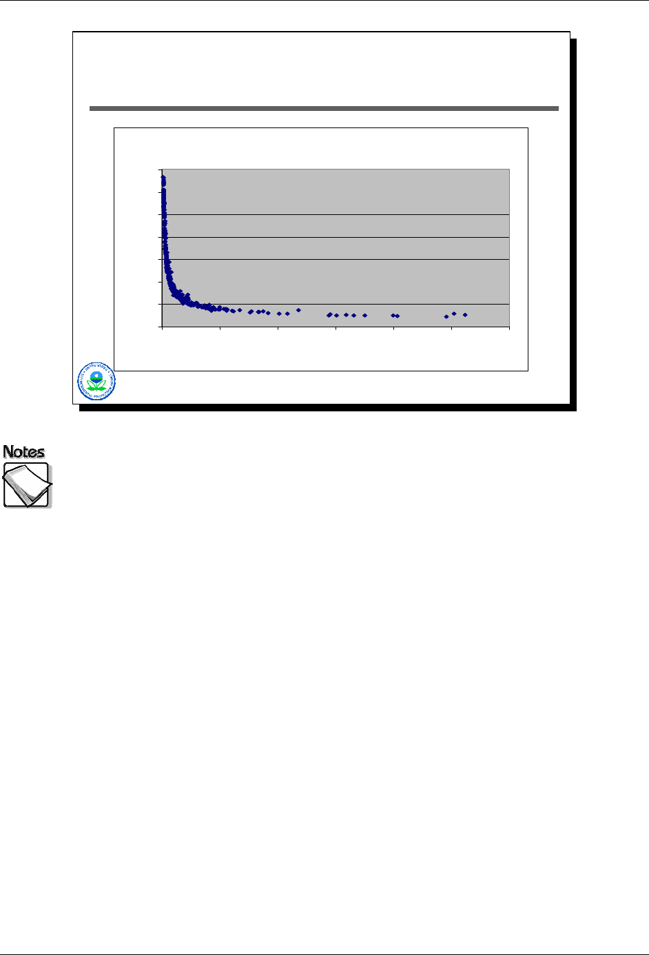
The graphic above illustrates the frequency of XRF responses when the element
is not present. Assume that a sample does not have an element present (or that
it is present at trace levels). If one were to take a measurement of the sample
with the XRF, the XRF would record a concentration present for that element just
because of the random nature of x-ray counting statistics. If one did a large
number of repeat measurements, one could generate a distribution or frequency
plot of those “random” concentrations such as is shown here, with a measurable
standard deviation. Notice that the frequency distribution is centered around
zero, indicating that this instrument is providing an unbiased estimate of the
concentration for the element of interest. Notice too that half the time the
instrument would report positive values, and half the time it would report negative
values…an important fact that will be discussed later. If one moves three
standard deviations up from zero and calls that the detection limit (consistent with
SW846 Method 6200), then almost 100% of the concentration values generated
when the element is not present would be less than the detection limit. In other
words, if the instrument records a result greater than this detection limit, then it is
very likely that in fact the element is present.
2-20 August 2008
XRF Web Seminar Module 2 – Basic XRF Concepts
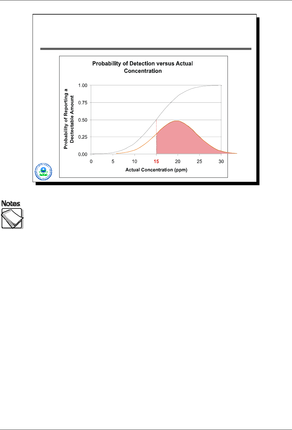
2-18
DL <> Reliable Detection
Stdev = 5 ppm
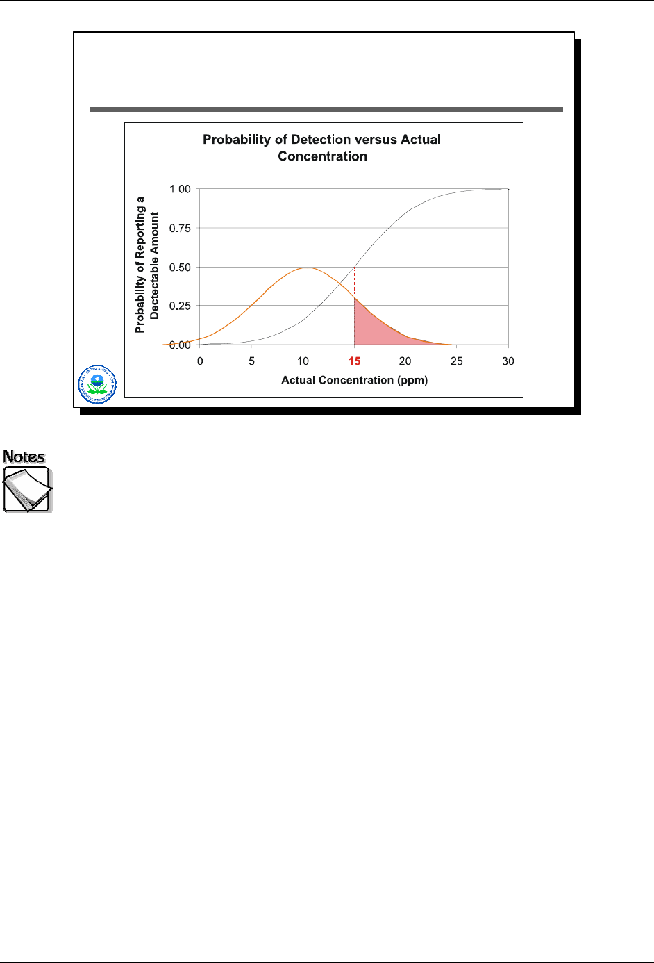
As defined and implemented, the detection limit for an XRF is not the same as
the concentration that can be reliably detected. The graphics on this and the
next two slides illustrate that fact. We start with the same scenario as the
previous slide, an element with a XRF detection limit of 15 ppm. In these slides,
the x-axis is actual concentration, while the y-axis is the probability the XRF will
detect the element. The three red bell-shaped frequency curves show what the
XRF response might be for three different actual concentrations (10 ppm, 15
ppm, and 20 ppm). The portion under the curves shaded red represents the
fraction of repeated measurements at that concentration that would have yielded
a result above the detection limit (15 ppm). As show in Slide 2-18 above, if the
actual concentration were 10 ppm, about a third of the measurements would
have yielded a “detection” (an XRF result > 15 ppm). The probability of reporting
a detection, as a function of actual concentration, is shown by the black S-
shaped curve.
August 2008 2-21
Module 2 – Basic XRF Concepts XRF Web Seminar
DL <> Reliable Detection
Stdev = 5 ppm
2-19
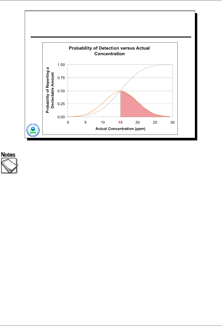
As shown in Slide 2-19 above, if the actual concentration were 15 ppm (at the
detection limit), the XRF would have detected the element only 50% of the time.
The probability of reporting a detection, as a function of actual concentration, is
shown by the black S-shaped curve.
2-22 August 2008
XRF Web Seminar Module 2 – Basic XRF Concepts
DL <> Reliable Detection
Stdev = 5 ppm
2-20
As shown in Slide 2-20 above, if the actual concentration was 20 ppm, the XRF
would have reported a detected value about two thirds of the time. In this
particular case, it is not until the actual concentration reaches 30 ppm (or twice
the DL) that the XRF will report a detectable value almost all of the time. The
probability of reporting a detection, as a function of actual concentration, is
shown by the black S-shaped curve.
August 2008 2-23

Module 2 – Basic XRF Concepts XRF Web Seminar
For Any Particular Instrument,
Detection Limits Are Influenced By…
Measurement time (quadrupling time cuts detection limits
in half)
Matrix effects
Presence of interfering or highly elevated contamination
levels
Consequently, the DL for any particular element will
change, sometimes dramatically, from one sample to the
next, depending on sample characteristics and operator
choices
2-21
Measurement time: The precision or reproducibility of a measurement will
improve with increasing measurement time. Increasing the count time by a factor
of 4 will provide 2 times better precision. Consequently increasing the count time
by a factor of 4 will cut detection limits by a factor of two. Of course, increasing
count time decreases sample throughput, so selecting the appropriate
measurement time is a trade-off between the desired detection limits and per-
sample measurement costs.
Matrix effects: Physical matrix effects result from variations in the physical
character of the sample. These variations may include such parameters as
particle size, uniformity, homogeneity, and surface condition. One way to reduce
error associated with variation in particle size is to grind and sieve all soil
samples to a uniform particle size. Differences in matrix effects can result in
differences in detection limits from one sample to the next.
Presence of interfering or highly elevated contamination levels: Chemical
matrix effects result from the differences in the concentrations of interfering
elements. These effects occur as either spectral interferences (peak overlaps) or
as x-ray absorption and enhancement phenomena. Both effects are common in
soils contaminated with heavy metals. For example, iron tends to absorb copper
x-rays, reducing the intensity of the copper measured by the detector, while
chromium will be enhanced at the expense of iron because the absorption edge
of chromium is slightly lower in energy than the fluorescent peak of iron. When
present in a sample, certain x-ray lines from different elements can be very close
in energy and, therefore, can cause interference by producing a severely
overlapped spectrum. The presence of interference effects will raise detection
limits.
2-24 August 2008
XRF Web Seminar Module 2 – Basic XRF Concepts
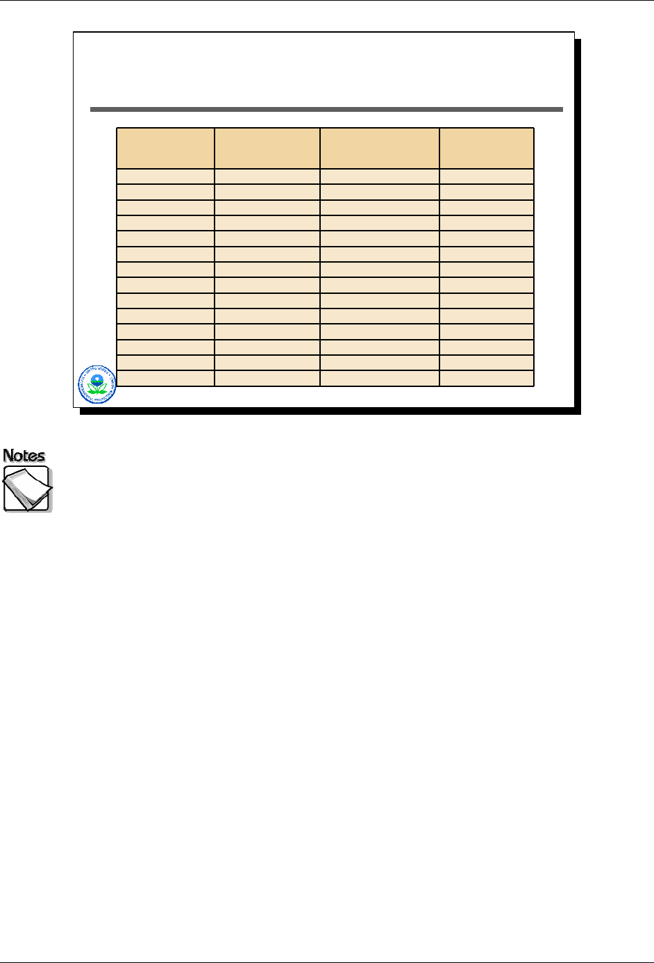
Examples of DL…
Analyte
Innov-X
1
120 sec acquisition
(soil standard –ppm)
Innov-X
1
120 sec acquisition
(alluvial deposits - ppm)
Innov-X
1
120 sec acquisition
(elevated soil -ppm)
Antimony (Sb) 61 55 232
Arsenic (As) 6 7 29,200
Barium (Ba) NA NA NA
Cadmium (Cd) 34 30 598
Calcium (Ca) NA NA NA
Chromium (Cr) 89 100 188,000
Cobalt (Co) 54 121 766
Copper (Cu) 21 17 661
Iron (Fe) 2,950 22,300 33,300
Lead (Pb) 12 8 447,000
Manganese (Mn) 56 314 1,960
Mercury (Hg) 10 8 481
Molybdenum (Mo) 11 9 148
Nickel (Ni) 42 31 451
2-22
The table illustrates the fact that detection limits can change dramatically from
sample to sample. Here we see three different sets of results from the same
Innov-X unit, in each case collected with a 120-second acquisition time. The
bold numbers in this table are actually quantified values (i.e., detects), while the
plain text numbers are detection limits for elements that were not detectable.
Results for three different samples are presented. The first is for a spiked matrix
(the spiked element is not present in this table). The second is for a background
soil sample taken from alluvial deposits. The third is for a highly contaminated
sample taken beneath a leaking waste sewer line at a chemical facility.
The effect of highly elevated lead and chromium on the detection limits for other
elements is severe. The detection limit for mercury jumps from around 10 ppm to
almost 500 ppm, a 50 times factor change.
One other note about these data. The concentration levels reported for
chromium and lead for the contaminated sample fall outside the calibrated range.
These values would and should be taken with a large dose of skepticism…the
levels of lead and chromium in this sample are undoubtedly extremely high, but
the ability of the XRF to accurately quantify them at these levels would be very
suspect.
August 2008 2-25

Module 2 – Basic XRF Concepts XRF Web Seminar
To Report, or Not to Report:
That is the Question!
Not all instruments/software allow the reporting of
XRF results below detection limits
For those that do, manufacturer often
recommends against doing it
Can be valuable information if careful about its
use…particularly true if one is trying to calculate
average values over a set of measurements
2-23
Not all instruments/software allow the reporting of XRF results below
detections limits: Some instruments and associated software do not allow the
reporting of measurement results that are below detection limits.
For those that do, manufacturer ofter recommends against doing it: For
those instruments that do allow reporting of results below detection limits, the
manufacturer usually advises against it. Within the chemistry analytical world,
the approach has been to not report values less than detection limits. Within the
radionuclide analytical world, the approach has been to report values less than
detection limits. The XRF is an analytical technique that has its roots in the
radionuclide world (e.g., gamma and alpha spectroscopy), but has applications to
the chemical world (e.g., elemental metals).
Can be valuable information if careful about its use . . . particularly true if
one is trying to calculate average values over a set of measurements:
Values below detection limits can be useful when calculating average values
over a set of measurements. If the instrument’s calibration is unbiased for low
levels of the element of interest, using measured values below the instrument’s
detection limits can yield more accurate assessments of average concentrations
that flagging readings as non-detects and substituting some arbitrary value such
as the detection limit, or half the detection limit, in average value calculations.
Great care and full disclosure are necessary when using values below detection
limits.
2-26 August 2008

XRF Web Seminar Module 2 – Basic XRF Concepts
XRF Data Comparability
Comparability usually refers to comparing XRF
results with standard laboratory data
Assumption is one has samples analyzed by both
XRF and laboratory
Regression analysis is the ruler most commonly
used to measure comparability
SW-846 Method 6200: “If the r
2
is 0.9 or
greater…the data could potentially meet definitive
level data criteria.”
2-24
Comparability usually refers to comparing XRF results with standard
laboratory data: The comparability of the XRF analysis is determined by
submitting XRF-analyzed samples for analysis at a laboratory. The XRF results
are then compared with the laboratory results.
Assumption is one has samples analyzed by both XRF and laboratory: The
confirmatory samples must be splits of well homogenized sample material. The
confirmatory samples should be selected from the lower, middle, and upper
range of concentrations measured by the XRF. They should also include
samples with element concentrations at or near the site action levels.
Regression analysis is the ruler most commonly used to measure
comparability: The results of the confirmatory analysis and XRF analyses are
usually evaluated with a least squares linear regression analysis.
SW-846 Method 6200: “If the r
2
is 0.9 or greater . . . the data could
potentially meet definitive level data criteria.”: Method 6200 states that the
method of confirmatory analysis must meet the project and XRF measurement
data quality objectives. The method also suggests that the r
2
for the results
should be 0.7 or greater for the XRF data to be considered screening level data.
Finally, the method states that if the r
2
is 0.9 or greater and inferential statistics
indicate the XRF data and the confirmatory data are statistically equivalent at a
99 percent confidence level, the data could potentially meet definitive level data
criteria.
August 2008 2-27
Module 2 – Basic XRF Concepts XRF Web Seminar
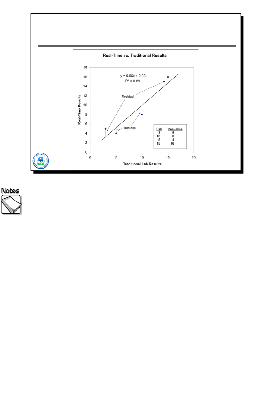
2-25
What is a Regression Line?
The scatter-plot in this slide illustrates how a regression analysis works. The
data in the lower-right table represents our collaborative data set: four samples,
with each having both a traditional laboratory result and a real-time result (e.g.
XRF). Plotting these data give us the scatter-plot shown. Assuming there’s a
linear relationship between results generated by the laboratory and results
generated by the real-time technique, the question is finding that linear
relationship.
The line shown represents the results from a regression using these data. The
regression line represents the “best fit” line. “Best fit” here is defined as the line
that minimizes the sum of the squared residuals. A residual is the vertical
distance separating a regression line and a data point.
2-28 August 2008
XRF Web Seminar Module 2 – Basic XRF Concepts
Regression Terminology
Scatter Plot: graph showing paired sample results
Independent Variable: x-axis values
Dependent Variable: y-axis values
Residuals: difference between dependent variable result
predicted by regression line and observed dependent
variable
Adjusted R
2
: a measure of goodness-of-fit of regression
line
Homoscedasticity/Heteroscedasticity: Refers to the size
of observed residuals, and whether this size is constant
over the range of the independent variable
(homoscedastic) or changes (heteroscedastic)
2-26
Regression terminology: The following are regression terms:
» Scatter Plot – graph showing paired sample results
» Independent Variable – x-axis values, usually the lab result
» Dependent Variable – y-axis values, usually the XRF result
» Residuals – difference between dependent variable result predicted by
regression line and observed dependent variable
» Adjusted R
2
– a measure of goodness-of-fit of regression line
» Homoscedasticity/Heteroscedasticity – refers to the size of observed
residuals, and whether this size is constant over the range of the independent
variable (homoscedastic) or changes (heteroscedastic)
August 2008 2-29
Module 2 – Basic XRF Concepts XRF Web Seminar
2-27
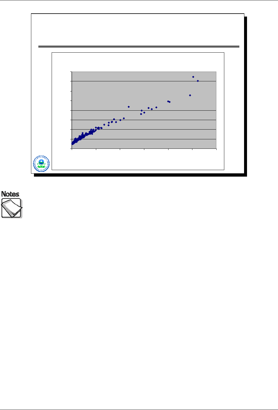
Heteroscedasticity is a Fact of Life
for Environmental Data Sets
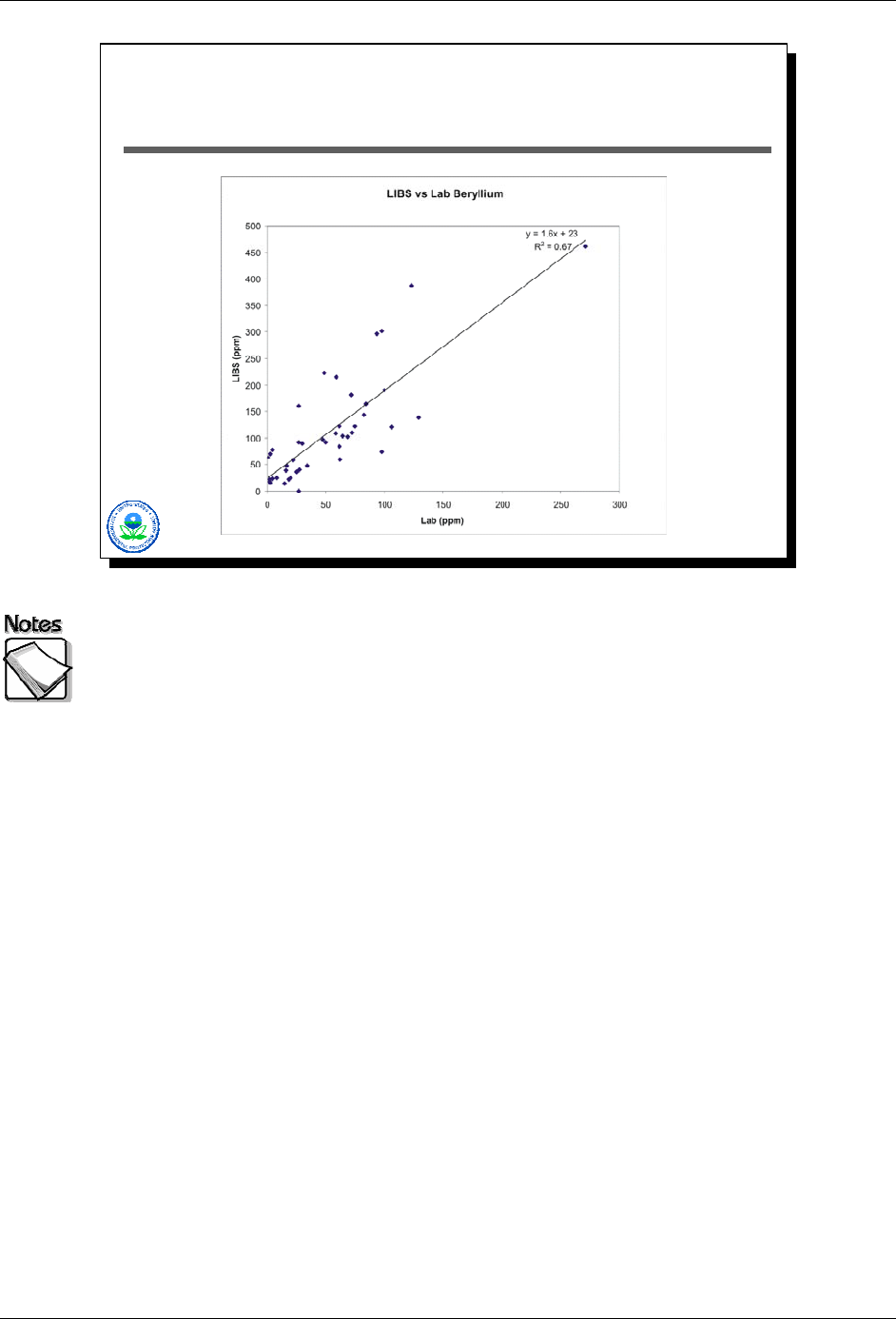
Heteroscedasticity is unfortunately a fact-of-life for environmental collaborative
data sets. The LIBS/laboratory scatter-plot illustrates the concept of
heteroscedasticity. We can fit a regression line to these data, with the resulting
line and its equation shown. The orange lines bracketing the regression line
above and below given a sense for how the size of residuals change as
concentrations increase. For low concentrations, the scatter-plot points are
tightly clustered around the regression line, giving rise to relatively small
residuals. As concentrations increase, the “scatter” of points around the line
steadily increases. The result is that residuals for higher-concentration points are
much larger than what they are for lower concentration values. This increasing
residual size as concentrations increase is called heteroscedasticity.
The concept is important because regression analyses often include UCL lines or
UTL lines that bracket the regression line. The problem with this is that UCL and
UTL calculations derived from a regression analysis are only valid if the
underlying data are homoscedastic…which environmental collaborative data
never are. The warning: beware of trying to extract too much from a regression
analysis’s results.
There is a simple physical explanation for heteroscedasticity in environmental
collaborative data…analytical error tends to increase as concentrations increase.
2-30 August 2008

XRF Web Seminar Module 2 – Basic XRF Concepts
Appropriate Regression Analysis
Based on paired analytical results, ideally from
same sub-sample
Paired results focus on concentration ranges
pertinent to decision-making
Non-detects are removed from data set
Best regression results obtained when pairs are
balanced at opposite ends of range of interest
2-28
Based on paired analytical results, ideally from same sub-sample: Such an
analysis should be based on paired results, ideally with the analytical work done
on the same sub-sample where possible to minimize the effects of sample
preparation. Poor comparability results are often the result of poorly prepared
samples and not analytical issues.
Paired results focus on concentration ranges pertinent to decision-making:
The paired results should focus on the concentration range pertinent to decision-
making. Often times field analytical methods have a more limited dynamic range
within which they provide accurate results. This means that it is unreasonable to
expect a good, strong linear relationship for two methods over the complete
range of concentrations (which may span several orders of magnitude) present at
a site. What is important is to determine whether such a relationship exists over
the range in which making decisions is important.
Non-detects are removed from data set: Non-detects should be removed from
a regression analysis because they will skew regression results.
Best regression results obtained when pairs are balanced at opposite ends
of the range of interest: The best regression results are obtained when the
data used are balanced, i.e., half are at the lower end of interest, and half are at
the higher end of interest. WARNING: unbalanced data sets (i.e., data sets
where most of the points are clustered at the low end with one or two high value)
will yield unstable and likely misleading regressions.
August 2008 2-31
Module 2 – Basic XRF Concepts XRF Web Seminar
Evaluating Regression Performance
No evidence of inexplicable “outliers”
Balanced data sets
No signs of correlated residuals
High R
2
values (close to 1)
Constant residual variance (homoscedastic)
2-29
No evidence of inexplicable outliers: There should be no evidence of outliers.
Outliers are points that clearly fall well away from the regression line and appear
to be different than the rest.
Balanced data sets: Data sets should be balanced.
No signs of correlated residuals: There should be no signs of correlated
residuals. Correlated residuals refer to the situation where a group of points
consistently fall above or below the regression line.
High R
2
values (close to 1): A good regression should have a high R
2
value,
preferably close to 1 (will range between 0 and 1).
Constant residual variance (homoscedastic): A good regression should also
have constant residual variance across the concentration range, or in other
words the data should be homoscedastic. Unfortunately for environmental
collaborative data sets, this is never the case.
2-32 August 2008
XRF Web Seminar Module 2 – Basic XRF Concepts
Example: XRF and Lead
Full data set:
» Wonderful R
2
» Unbalanced data
» Correlated residuals
» Apparently poor calibration
Trimmed data set:
» Balanced data
» Correlation gone from residuals
» Excellent calibration
»R
2
drops significantly
2-30
Here’s an example based on XRF analyses of lead in soil samples. The top
graphic shows a scatter plot based on the complete data set collected. The
regression line has a wonderful R
2
value, but has several obvious visual
deficiencies. These include unbalanced data (most of it clustered at the low end
with only two points at the high end), correlated residuals, and what appears to
be a poor calibration for the XRF based on the slope of the line.
The second data set has had its data trimmed to include only those
concentrations that fall within the range truly of interest from a decision-making
perspective. These data are balanced across the concentration range of interest.
The correlations are gone from the residuals. The slope corresponds to what
one would expect from a calibrated XRF. Note that the R
2
value is actually less,
though, then the first example, even though the second regression is clearly
superior, underscoring the problems with simply using R
2
values as a measure of
regression performance and hence field analytic data quality and usability.
Also, in the second scatter plot the spread of the data around the line increases
as concentrations increase. This is called heteroscedasticity, and indicates that
the variance of the data is not constant over the range of observed
concentrations. The presence of heteroscedasticity is a given in environmental
data, and complicates the interpretation of regression results. Therefore,
interpreting UCLs and UTLs for regression lines when heteroscedasticity is
present should be done very carefully.
August 2008 2-33

Module 2 – Basic XRF Concepts XRF Web Seminar
Converting XRF Data for Risk
Assessment Use
Purpose: making XRF data “comparable” to lab data for
risk assessment purposes
To consider:
» Need for “conversion” may be an indication of a bad
regression
» XRF calibrations not linear over the range of
concentrations potentially encountered
» Extra variability in XRF data not an issue (captured in
UCL calculations when estimating EPC)
» Contaminant concentration distributions are typically
skewed… lots of XRF data may provide a better
UCL/EPC estimate than a few lab results even if the
regression is not great
2-31
Purpose: Some times XRF data are “converted” using a regression line to make
them “comparable” to laboratory data. One might do this if one wants to pool the
XRF data with lab data for risk assessment purposes.
To consider: Before “transforming” XRF data in this fashion, the following
should be considered:
» Need for “conversion” may be an indication of a bad regression
» XRF calibration are not linear over the range of concentrations potentially
encountered
» Extra variability in XRF data should not be an issue (captured in upper
concentration limit (UCL) calculations when estimating the exposure point
concentration (EPC))
» Contaminant concentration distributions are typically skewed . . . a large
volume of XRF data may provide a better UCL/EPC estimate than a few
laboratory results even if the regression is not great.
2-34 August 2008

XRF Web Seminar Module 2 – Basic XRF Concepts
A Cautionary Example…
Four lab lead results: 20, 24, 86, and 189 ppm
ProUCL 95%UCL Calculations:
»Normal: 172 ppm
»Gamma: 434 ppm
»Lognormal: 246 – 33,835 ppm
»Non-parametric: 144 – 472 ppm
Four samples are not enough to either
understand the variability present, or the
underlying contamination distribution
2-32
This example shows that four samples are not enough to either understand the
variability present, or the underlying contamination distribution, no matter how
“high quality” the laboratory data are. If the action level for this site were 400
ppm, the decision about whether the area posed a risk or not would be
ambiguous. A larger volume of measurements, even if they were from an XRF
with analytical quality not quite as good as the lab’s, would provide a better
understanding of variability and contaminant distribution, and consequently a
better UCL estimate, assuming the XRF was properly calibrated for the element
of interest.
August 2008 2-35
Module 2 – Basic XRF Concepts XRF Web Seminar
2-33
Will the “Definitive” Data Please
Stand Up?
One of these scatter plots shows the results of arsenic from two different
ICP labs, and the other compares XRF and ICP arsenic results.
Which is which?
These two scatter plots show paired data results for arsenic. In one case,
samples first analyzed by XRF were then sent off for ICP analyses. In the other
case, the same sample was split and sent for ICP analyses to two different labs.
Which of these two corresponds to the ICP/ICP comparison, and which to the
XRF/ICP comparison?
The answer is that the scatter plot on the right compares XRF to ICP, while the
scatter plot on the left shows ICP versus ICP results for two different labs for the
same set of samples.
The take home point is quite simple. Traditional analyses are often treated as
though they are “definitive” and free from error. When the results of an
alternative analysis such as an XRF are compared to those from a traditional lab,
any differences observed are attributed to poor performance on the alternative
analysis’s part. The reality is not so simple. Traditional analyses also include
“errors” that need to be recognized.
2-36 August 2008
2-34
XRF Web Seminar Module 2 – Basic XRF Concepts
Definitive Data, Please Stand Up!
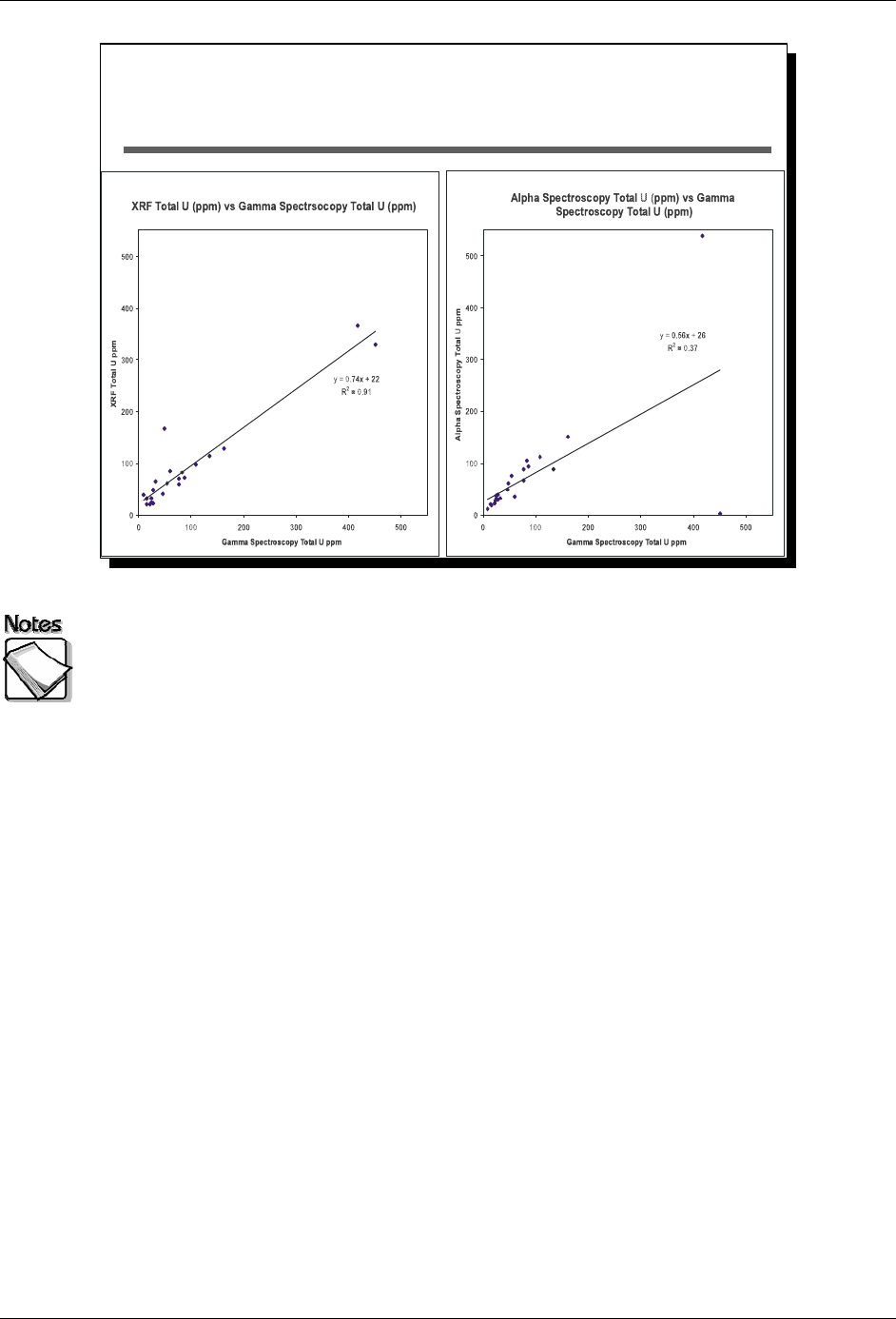
2-34
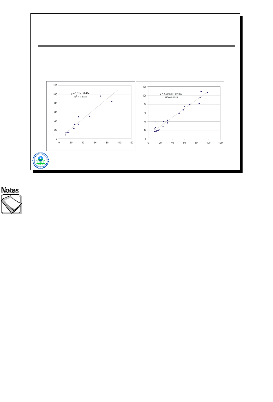
This slide shows results from a set of samples analyzed with three different
methods for uranium, via XRF (very limited sample preparation), gamma
spectroscopy (sample preparation, but no extraction), and alpha spectroscopy
(sample preparation with extraction required). The plot on the left compares XRF
and gamma spectroscopy data with a resulting R
2
of 0.91. The plot on the right
compares alpha spectroscopy and gamma spectroscopy data with a resulting R
2
of 0.37. Both gamma spectroscopy and alpha spectroscopy are well-established
methods for measuring uranium in soils. In this particular case, if the XRF had
just been compared to alpha spectroscopy results, the likely conclusion would
have been that there were performance problems with the XRF. The availability
of gamma spectroscopy data as well helped to identify alpha spectroscopy as the
problem for at least two of the samples.
August 2008 2-37

Module 2 – Basic XRF Concepts XRF Web Seminar
Take-Away Comparability Points
Standard laboratory data can be “noisy” and are
not necessarily an error-free representation of
reality
Regression R
2
values are a poor measure of
comparability
Focus should be on decision comparability, not
laboratory result comparability
Examine the lab duplicate paired results from
traditional QC analysis - The split field vs. lab
regression cannot be expected to be better than
the lab’s duplicate vs. duplicate regression
2-35
Standard laboratory data can be “noisy” and are not necessarily an error-
free representation of reality: It is a mistake to believe that standard laboratory
data are free of errors. This can be seen when laboratory analyses from two
different laboratories are compared to one another in the same way that XRF and
laboratory data are compared.
Regression R
2
values are a poor measure of comparability: Regression
performance should be judged using a number of factors, not just the R
2
value.
Focus should be on decision comparability, not laboratory result
comparability: Decision comparability judges whether or not data is suitable for
the decision at hand. XRF data may be suitable for decisions about whether an
action level has been exceeded or for calculating UCL/EPC even when the
regression is not perfect.
Examine the lab duplicate paired results from traditional QC analysis:
Frequently the regression from duplicate paired results is poor. It is
unreasonable to expect the split field (XRF) versus laboratory regression to be
better than the laboratory’s duplicate versus duplicate regression.
2-38 August 2008

XRF Web Seminar Module 2 – Basic XRF Concepts
What Affects XRF Performance?
Measurement time – the longer the
measurement, the better the precision
Contaminant concentrations – potentially
outside calibration ranges, absolute error
increases, enhanced interference effects
Sample preparation – the better the sample
preparation, the more likely the XRF result will be
representative
(continued)
2-36
Measurement time: The longer the measurement time or count time, the better
the precision will be.
Contaminant concentrations: Contaminant concentrations may be outside of
the calibration ranges. Other contaminants may cause interference effects.
Sample preparation: The better the sample preparation, the more
representative the XRF results will be of actual conditions.
August 2008 2-39

Module 2 – Basic XRF Concepts XRF Web Seminar
What Affects XRF Performance?
Interference effects – the spectral lines of
elements may overlap
Matrix effects – fine versus coarse grain
materials may impact XRF performance, as well
as the chemical characteristics of the matrix
Operator skills – watching for problems,
consistent and correct preparation and
presentation of samples
2-37
Interference effects: The spectral lines of elements may overlap distorting
results for one or more elements.
Matrix effects: Physical matrix effects, such as fine versus course grain
materials, may impact XRF performance. In addition, chemical characteristics of
the matrix may also impact XRF performance.
Operator skills: The level of operator skill can affect XRF performance. The
operator should watch for problems and should practice consistent and correct
preparation and presentation of samples.
2-40 August 2008

XRF Web Seminar Module 2 – Basic XRF Concepts
What Are Common XRF
Environmental Applications?
In situ and ex situ analysis of soil samples
Ex situ analysis of sediment samples
Swipe analysis for removable contamination on
surfaces
Filter analysis for filterable contamination in air
and liquids
Lead-in-paint applications
2-38
August 2008 2-41

Module 2 – Basic XRF Concepts XRF Web Seminar
Recent XRF Technology
Advancements…
Miniaturization of electronics
Improvements in detectors
Improvements in battery life
Improved electronic x-ray tubes
Improved mathematical algorithms for
interference corrections
Bluetooth, coupled GPS, connectivity with PDAs
and tablet computers
2-39
Recent XRF technology advancements: The following advancements in XRF
technology have improved the performance of the technology:
» Miniaturization of electronics – this has made the instruments more portable
» Improvements in detectors – with a corresponding lowering of detection limits
» Improvements in battery life – which increases sample throughput by
reducing instrument downtime and improves general field application
» Improved electronic x-ray tubes – which improves performance of the units
» Improved mathematical algorithms for interference corrections – which
expands the applicability of the technology
» Bluetooth, coupled GPS, connectivity with PDAs and tablet computers –
which enhances data collection, management, and storage
2-42 August 2008
XRF Web Seminar Module 2 – Basic XRF Concepts
…Contribute to Steadily Improving
Performance
Analyte
DL in Quartz Sand by
Method 6200
(600 sec – ppm)
TN 900 (60 to
100 sec) – ppm
Innov-X
1
120 sec acquisition
(soil standard – ppm)
Antimony (Sb) 40 55 61
Arsenic (As) 40 60 6
Barium (Ba) 20 60 NA
Cadmium (Cd) 100 NA 34
Chromium (Cr) 150 200 89
Cobalt (Co) 60 330 54
Copper (Cu) 50 85 21
Iron (Fe) 60 NA 2,950
Lead (Pb) 20 45 12
Manganese (Mn) 70 240 56
Mercury (Hg) 30 NA 10
Molybdenum (Mo) 10 25 11
Nickel (Ni) 50 100 42
2-40
This last table shows the results of XRF technology improvements over the
years. The first data column shows XRF detection limits as reported in Method
6200 in the best of conditions - quartz sand with a 600 second acquisition. The
second column shows the performance of a TN 900 XRF in the mid to late 1990s
(the table containing these results is dated 1998) with a 60 to 100 second
acquisition. One would expect these values to be less than half of what is
reported if a 600 second acquisition time had been used. The last column shows
data collected with an Innov-X unit in 1996 for a spiked soil standard (the spiking
element is not present in this table). Results in bold indicate actual measured
data. Plain text results are reported detection limits. The detection limit
differences are marked for a number of samples. For example, in the case of
arsenic the Innov-X detection limit is one tenth that of the TN 900 back in the
1990s. This improvement is not vendor-specific…in fact all vendors of portable
XRF technologies have made significant strides in improving instrument
performance in the last decade. One would expect those improvements to
continue and be reflected in falling detection limits and better handling of
interference effects.
August 2008 2-43

Module 2 – Basic XRF Concepts XRF Web Seminar
2-41
Q&A – If Time Allows
2-44 August 2008
